Explainable AI for ransomware resiliency with SHAP

Machine learning models are great tools to solve those complex problems not easily handled by conventional programming methodologies. The ability to solve large-scale problems using just historical data comes at the cost of transparency in terms of the results. The models are “black boxes” to the ML teams and end-users. Explaining why a model makes a prediction can be as important as the model accuracy itself in many applications. 

At Druva Labs, while working on multiple machine learning models for multiple use cases, the one requirement that was always at the top of everyone’s mind was “how do we ensure trust in the predictions of the model to the end-user?” While we were ensuring model performance remained above the acceptance criteria set by stakeholders, the ability to explain why a prediction was made by the model was crucial to end-users. 

In this blog post, we will walk through one of the instances at Druva Labs where model explainability was an important aspect of the machine learning solution for us, and how SHAP enabled us in achieving the desired results. We will also provide a brief overview of anomaly detection and machine learning model explainability using SHAP. At Druva Labs, we came across multiple use cases deemed fit for a machine learning solution; we worked on problems such as supervised regression, unsupervised anomaly detection, and many more.

The explainability depends heavily on the type of problem and the modeling algorithms. It could be as simple as using coefficients from linear regression models and rules extracted from decision trees to complex explanation methods used for ensemble models such as Random Forest. 

Fig:1. Post hoc Explanation System. 

Model Explainability Overview

Explanation or interpretability in AI aims at creating a set of techniques that produce explainable models that are easily understood and trusted. Highly interpretable models make it easier to comprehend why certain decisions or predictions were made. 

Some algorithms are intrinsically easier to explain than others, such as decision trees. On the other hand, some algorithms require post hoc explainability because they are not readily interpretable. In order to enhance explainability in such cases, diverse techniques can be employed like text explanations, visual explanations, local explanations, feature relevance, etc. A brief introduction to the area of XAI (explainable AI) can be found in a previous blog post by the Druva Labs team. 

SHAP — SHapley Additive exPlanations 

The idea behind using SHAP for model interpretability is based on Shapley values. Here, we believe a prediction can be explained by considering each feature value as a player in a game where the prediction is the winning prize. Shapley values — a method from coalition game theory — allow us to fairly distribute contributions to features.

Consider the example of house price prediction — we have several features of houses and the selling price is to be predicted. If a model has predicted the selling value as 300k based on feature values, such as the number of bedrooms, surface area, etc., then we’ll want to know how much has each feature contributed to the prediction. If the model is a simple linear regression, then the feature weights are the contributions. For more complex models, better methods are needed. Explainability methods like LIME (local interpretable model-agnostic explanations) attempt to fit local models to estimate the feature contributions. The Shapley value is another solution for complex models. 

For the Shapley value method, we assume the game is the task of price prediction for a single instance of the dataset, while the features are the players, and the prize is the actual prediction of this instance minus the average prediction of price across all instances. The players collaborate to win the prize, and the Shapley value is the average of all marginal contributions to all possible collaborations of players/features. The difference in the value of marginal contributions of a feature when added to coalitions is averaged across all observations and represents the Shapley value of that feature. 

If we estimate the Shapley values for all features, we can get the distribution of predictions among the features. 

SHAP and Supervised ML

The Shapley value works for both classification and regression. For demonstration purposes of classification tasks using the iris dataset, below we explain the output from different models such as KNN, SVM, neural networks, etc. 

The SHAP python library allows us to generate brilliant visualizations to explain the model outputs. For example, in order to explain a single prediction we can use the below visualization:

Fig:2(a). Observation Explanation.

In the above figure, we can see the features and their impact on the decision. The blue arrows define the features that helped make the SHAP score lower, and the red arrows (not present in this instance) suggest features that raise the score. 

We can also explain all predictions for the test set using the following visualization: 

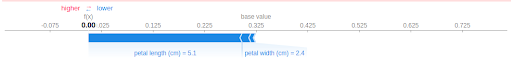
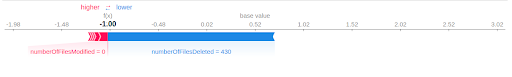
Fig:2(b). Observation Explanation.

Data Resiliency — An Unsupervised Anomaly Detection Initiative from Druva Labs

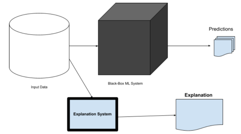
As we covered previously, using SHAP for model explanation can offer helpful insights into model behaviors globally (for the entire dataset) as well as locally (per observation). For the supervised ML algorithms SHAP support is sufficient, things get tricky when we come to unsupervised machine learning techniques. 

One of our Machine learning initiatives is an anomaly detection system for data resilience, which is a log-based, dynamic outlier detection method. We evaluated many algorithms for this purpose including distance-based, density-based, and clustering algorithms, and one of the top contenders is the tree-based isolation forest. Although achieving good model accuracy with low false-positive predictions is the primary goal, providing explainability in terms of feature contributions for each prediction to the end-users was also a major requirement. 

In the following section, we’ll explore how we addressed this requirement with some example visualizations. 

Model Explainability using SHAP for Isolation Forest

During our evaluation, we understood how isolation forest can be utilized for multidimensional anomaly detection. We tested it alongside many other anomaly detection algorithms, but due to its simple structure and low runtime complexity, isolation forest was a popular choice. For providing model explainability, we utilized the SHAP python library. The following sections will walk through the isolation algorithm and demonstrate how we used SHAP for explainability. 

Anomaly Detection with Isolation Forest 

Isolation forest is a popular unsupervised anomaly detection algorithm. It detects anomalies using isolation rather than trying to model normal points. Isolation forests are built using decision trees. 

The basic workflow for isolation forest-based anomaly detection is as follows:

1. Randomly select a feature from the given set of features.
2. Randomly select a split value for the feature between the minimum and maximum value. 
3. The data is partitioned on the split value of that feature.
4. Continuous recursive partitioning is done until an instance is isolated. 
5. The path length from root to terminating node is equivalent to the number of splittings, and an anomalous instance will have a shorter path length or fewer splittings for isolation. 
6. The path length averaged over a forest of many such isolation trees is a measure of the normality of data and our decision function. 

SHAP for Isolation Forest 

The explainability of an anomaly detection algorithm like isolation forest answers the following questions: 

• Why is a particular observation considered anomalous by the model?
• Which features contributed to identifying an observation as an anomaly and which didn’t?
• How can the output of the model on a real-world dataset be interpreted?

The interpretation can be either global or local. In global, we need to explain the model as a whole and understand which features play a more relevant role in the model. Whereas local interpretations look at individual observations and explain the feature contributions that resulted in the given prediction for that observation. 

For the purpose of this blog, let’s consider a sample of the dataset we created for the proof of concept phase of our unsupervised anomaly detection for unusual activity detection use case.

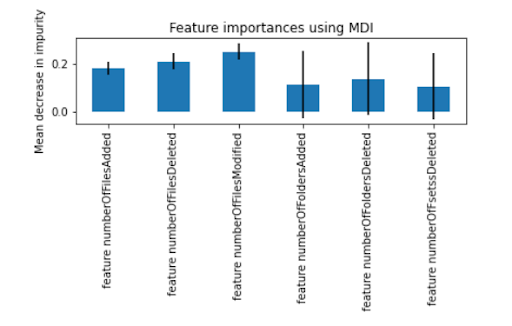
In this sample dataset, there are 1,000 observations and many features, but for simplicity, here we selected only six top features. The features represent user activity detected during a backup, such as count of files added, count of files deleted, count of files modified, count of folders added, count of folders deleted, and count of files renamed. Our objective was to use these features as representatives of user activity and detect any unusual user behavior that could have been caused by human error, malicious intent, or a malware/ransomware attack on the system. 

For unsupervised anomaly detection, we fit an isolation forest model using the implementation by Sklearn library. The labels generated by the models are stored in a new column, where -1 represents an anomalous, and 1 represents a normal observation. We then used SHAP to explain the predictions for both local and global interpretability. 

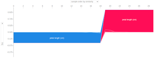
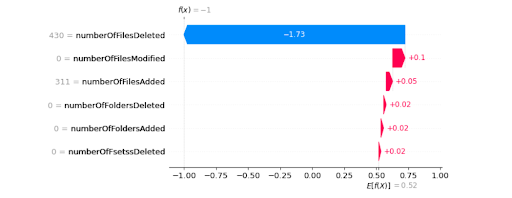
Explain Single Predictions

Once a prediction is made by the trained unsupervised anomaly detection model we can compute SHAP values. We used TreeExplainer and Explainer objects for our isolation forest model. Below are some of the analyses we could perform using SHAP.

Fig:3. Waterfall plot for a single observation labeled as anomalous by the model. Here the blue marked feature indicates the magnitude and direction of the contribution of the major contributor feature. The red marked features contributed to pushing the observation toward normal behavior. 

In Fig:3, for a single prediction, the contributions of each feature along with their degree of influence and direction are shown. The direction to the left and in blue indicates influence towards being anomalous for that feature. The right direction and red color bars indicate the features’ influence on the observation being non-anomalous. 

Another local explainability visual based on SHAP values calculated for each observation is the force plot, shown in Fig:4. It indicates the major contributor features in blue and also the features that influence the prediction of a normal data point in red. 

Fig:4. Force plot of a single observation labeled as an anomaly by the model. The blue arrow indicates the feature numberoffilesdeleted contributed majorly towards the observation being an anomaly. 

Explain Single Feature

We can explain individual features using the dependency scatter plot colored by an interaction feature as shown below. 

Fig:5. Scatter plot showing the explanation of a feature.

In Fig: 5, on the X-axis the feature values are shown; on the Y-axis, the SHAP-values are plotted. This shows how the model depends on the considered feature.

We can see summary plots too, that present the impact of high vs. low value of the features for an observation. 

Global Interpretability

Here we want to display the feature importance of the entire dataset’s predictions. Fig:6 below is the summary plot. It indicates what features, along with their high vs. low values, are influencing the prediction to be anomalous or normal. 

Fig:6. Summary plot of the model. Red points indicate high values for the feature and blue indicates low — here almost all features have more anomalies with high values.

We can see from the diagram the major influencer features for the predictions on the entire dataset. For example, the feature numberOfFilesModified, when high in magnitude yields large negative SHAP values, and when low in magnitude yields small positive SHAP values. This indicates for the feature numberOfFilesModified high magnitude values contribute more towards anomalous labels as compared to low magnitude values. The same information can be clearly seen using a bar plot. 

Fig:7. Bar Plot of all features and their contribution for the model.

We validated the SHAP results above using a simple workaround, where we trained a supervised classifier (random forest) on the isolation forest results and took feature importances. The feature importances extracted from a random forest model are shown below:

Fig:8. Feature importance from supervised classifier using random forest, trained on the same data as isolation forest model and labels being the isolation forest results.

As seen in the above figure, the contributions we derived from SHAP match the feature importances we got from random forest. The results may vary based on the size of the data and also on the domain the data comes from. We chose such a workaround due to the lack of availability of a labeled dataset. 

Conclusion

In this blog post, we took a journey through machine learning explainability, and witnessed, in brief, how the Druva Labs team solves complex problems at scale — such as anomaly detection and supervised/unsupervised machine learning. We also observed how important model interpretability is to the stakeholders as well as ML teams. 

We are providing explainability for our AI/ML models to establish trust and understanding for end-users. Based on experience with multiple use-cases targeted toward a variety of stakeholders, we can confidently claim that machine learning explainability will continue to be one of the most important features of any machine learning project. Hence, our recommendation to readers is to consider model interpretability as part of the data science process while evaluating modeling algorithms. A simple but explainable model might just be the better choice for your team over a high-performance black-box model. 

Next steps

Learn more about the technical innovations and best practices powering cloud backup and data management. Visit the Innovation Series section of Druva’s blog archive.

Join the team!

Looking for a career where you can shape the future of cloud data protection? Druva is the right place for you! Collaborate with talented, motivated, passionate individuals in a friendly, fast-paced environment; visit the careers page to learn more.

About the author

Anurag Singh Waliya is a Senior Staff ML Engineer for Druva Labs. As part of the Labs team, Anurag is focused on next-generation initiatives using machine learning that will greatly impact customer business goals. His interests include learning about emerging technologies and helping create awareness regarding use of data science solutions for social good.