Neural Networks Visualization + Interactive Training

Neural networks are exciting new trends in technology because they provide practical forms of machine intelligence that can solve many use cases within different technology domains — from data search optimization to data storage optimization. However, when we start to dive deeper to understand the concepts of neural networks, many developers find themselves overwhelmed by the associated mathematical models and formulas. To solve this problem, I will introduce you to a practical approach to easily understand neural networks through visualization using TensorFlow Playground.

What is TensorFlow Playground?

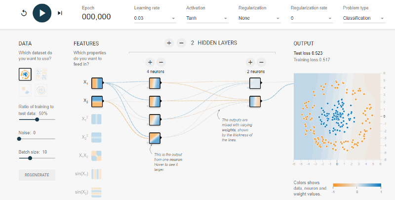
Google developed an open-source application that is well known for explaining how neural networks work in an interactive way: TensorFlow Playground. TensorFlow Playground is a web application that is written in d3.js (JavaScript), and it allows users to test the artificial intelligence (AI) algorithm with the TensorFlow machine learning library.

Interactive UI of TensorFlow — neural network playground

Let’s look at some TensorFlow Playground demos and how they explain the mechanism and power of neural networks.

Neural network dictionary

Before starting the demos, here are some crucial building blocks of the deep learning model. Neural networks consist of three layers of nodes:

• Input layer: This is the first layer of the neural network which passes the information to subsequent layers without performing any computational tasks.
• Hidden layer: This consists of one or more layers and acts as the connection between the input and output layer. These layers perform all the computational work.
• Output layer: This layer is responsible for transferring the data to the outside world.

Each layer can have one or many nodes. The neural network having multiple hidden layers with one or more neurons is called a ‘Deep Neural Network.’ This type of model is used in various applications of machine learning such as machine translation, image processing, speech recognition, image recognition, etc.

The parameters of neural networks that we can play with in these demos are:

• Epoch: An epoch is one complete cycle when the entire dataset is passed forward and backward through the neural network once.
• Learning rate: Learning rate is a configurable hyperparameter (the properties/parameters that govern the whole Neural Network training visualization process) used in the training of neural networks that has a small positive value. The learning rate ranges from 0.00001 to 10 in the Tensorflow playground. It controls how quickly the model is adapted to the problem. Smaller learning rates require more training epochs given the smaller changes made to the weights each update, whereas larger learning rates result in rapid changes and require fewer training epochs.
• Activation function: This is the function in an artificial neuron that delivers an output based on inputs. ReLU, Tanh, Sigmoid, and Linear are some available activation functions in the Tensorflow playground. The output of each function is used as an input in the next function in each epoch until we get the desired solution.
• Regularization rate: This is a technique used for tuning the activation function by adding an additional penalty term in the error function. The value of the regularization rate varies from 0 to 10 in the Tensorflow playground.
• Problem type: Problem type is broadly classified into two parts: classification and regression. Classification problems are those problems that have categorical output, e.g., an artificial neural network used to identify dog vs cat. In these scenarios, the output is either of the two categories, i.e cat or dog. In regression problems, the output is a numerical value ranging from starting and ending point (e.g., an artificial neural network used to identify dog vs cat, the output can also be shaped as a percentage match as dog or cat. In this scenario, the output lies between 0–100).
• The ratio of the training and testing sets: Every given dataset is divided into categories: testing and training sets. The training set is the set of data that is used to train the neural network to get the desired output. The testing set is the set of data that is used to test the model prediction capability, on an unseen data set. We usually set that ratio to 70/30 or 80/20.
• Noise: Noise is a distortion in data, that is unwanted by the perceiver of data. Adding noise to inputs is like telling the network to not change the output in a ball around your exact input.
• Batch size: This refers to the number of training examples or data points utilized in one epoch. For example, the batch size is usually between 10 and 1000. Batch size is usually fixed during training and inference; however, the TensorFlow Playground does permit dynamic batch sizes.
• Features: Features are the properties of the node or neuron that we want to feed in during the artificial neural network generation. There are a number of properties to choose from in the Tensorflow Playground.
• Hidden layer: These are layers that are located between the input and output layer, in which the function applies different weights to the inputs and directs through an activation function as the output. There can be one or many hidden layers with one or many nodes attached to it.
• Output layer: This is the last layer in the artificial neural network generation that produces the output of neural nets.

Shallow and Deep Neural Networks.

Understanding neural networks

In this section, we will perform a few experiments to better understand neural networks.

We will start with a simple classification-problem example and then proceed to our experiment with complex data sets. In this, the data set consists of orange and blue points in the form of two concentric circles. This will help us to better understand the concept of neural networks. We have used the following parameters for our run:

• 2 Hidden Layer with 4 Neurons in the first layer and 2 Neurons in the second layer
• Activation function: ReLU
• Learning rate: 0.003
• Regularization: None
• Regularization rate: 0

Problem type: Regression

According to the demonstration above, we can see that with the learning rate = 0.03 and the ReLU activation function, in just 150 epoch we get a clear differentiation in the shape of a hexagon in between blue and orange points.

It’s important to note that the difference in the thickness of lines joining different neurons defines the difference in the weight of the feature. The thicker the line joining the neurons means that more weight is given to that feature and vice versa.

Neural network demo experiments

In the following neural network experiments, we will use an interesting data set, which will help us to test our concepts and perform various experiments to help us to find the best model possible.

The data set we will use consists of orange and blue points in the form of two spiral rings as shown in the diagram below.

Neural network experiment 1

Let’s train a neural network and see whether it can separate a complex data set or not. We will start with a basic setup with just one hidden layer:

• 1 Hidden Layer with 4 Neurons each
• Activation function: Tanh
• Learning rate: 0.003
• Regularization: None
• Regularization rate: 0
• Problem type: Regression

In this demo, we can see that the neural network is trying, but it's really struggling. After running for a while, it’s starting to get there and is converging some parts of blue and orange areas. The problem with neural networks is that it does not have enough neurons to separate this complex structure.

Neural network experiment 2

In this run, we will add another layer of the hidden layer with four neurons, and discover if that would help us find the right solution. We will keep the other parameters as is:

• 2 Hidden Layer with 4 neurons each
• Activation function: Tanh
• Learning rate: 0.003
• Regularization: None
• Regularization rate: 0
• Problem type: Regression

We can see the neural network is doing more complicated things than before because it has more neurons to work with. The separation between blue and orange areas is more prominent and it has improved in comparison to our last run. But it’s still not where it needs to be.

Neural network experiment 3

Let’s add some more layers and neurons and make it a more conventional neural network design with input layer data going into 8 neurons on the first hidden, 6 in the second, 4 in the third, and 2 in the last layer to produce the binary output that we want. We will have a typical tree-like structure for our neural network. We will be keeping the rest of the parameters the same as before:

• 4 Hidden Layer with 8 neurons on the first, 6 in the second, and 4 in the third and 2 in the fourth layer
• Activation function: Tanh
• Learning rate: 0.003
• Regularization: None
• Regularization rate: 0
• Problem type: Regression

The convergence rate increased drastically. The results, in which we were receiving 900+ epochs in the previous runs, are now receiving around 400 epochs with much better separation in the orange and blue zones. It’s attaining the spiral and the tendrils are getting weaker and weaker, but the orange zone is overfitting in some areas and still not there yet completely. Overfitting happens when a model learns the detail and noise in the training data to the extent that it negatively impacts the performance of the model on new data and we can clearly see that in our case that the orange zone is overfitting on some blue zones.

Neural network experiment 4

With 20 neurons, we have attained fairly decent results. The next parameter that we must change is the activation function because it is the most important role for neural networks. We have been using Tanh for our experiments until now. However, now we will use a more powerful activation function: ReLU.

ReLU stands for the rectified linear unit and is a type of activation function. Mathematically, it is defined as y = max(0, x). It is currently the most utilized activation function. Another advantage of ReLU is that it is computationally less expensive than Tanh.

• 4 Hidden Layer with 8 neurons on the first, 6 in the second, and 4 in the third and 2 in the fourth layer
• Activation function: ReLU
• Learning rate: 0.003
• Regularization: None
• Regularization rate: 0
• Problem type: Regression

Finally! We achieved our desired result. The speed of convergence is much faster on the same neural network with the ReLU activation function. We are able to see a well-defined spiral structure after only 350 epochs. The distinction between the orange and the blue zone is significant. There is a little bit of overfitting, but we created our spiral shape.

Next steps

There are many more parameters that we could test, and we could observe different behaviors with different types of data. It’s great to see the desired results and have a concrete understanding of each and every parameter so that we could build better neural networks in the future with perfect parameter tuning. More importantly, we can achieve all of this in our browser without having any external library or computation power in our machine. This blog is just the beginning for those who want to explore and understand the power of neural networks. Happy tinkering.

Learn more about technological advancements in AI that are emerging as real-world applications.